Network Interpretability of Lung X-rays
In this tutorial, we demonstrate visualizing network interpretability through a classification task. We will make use of MONAI, a PyTorch-based deep learning framework for medical imaging. Specifically, we’ll adapt of one of the existing tutorials and show how the xaitk-saliency package can complement the current interpretability functionality in MONAI.
The data are a set of X-rays collated from a variety of sources. The labels used are:
normal (the absence of the following classes)
pneumonia
covid
Using the MONAI package, we will demo the use of GradCam and occlusion sensitivity to interpret the trained network’s classification choices. Using the xaitk-saliency package, we will demo the use of occlusion sensitivity with both sliding window and randomized input sampling (RISE) perturbation.
Table of Contents
To run this notebook in Colab, use the link below:
![]()
Note, this is a compute-intensive notebook and the free resources provided by Colab may not be sufficient for successful execution within Colab’s runtime limits.
Set Up Environment
Note for Colab users: after setting up the environment, you may need to “Restart Runtime” in order to resolve package version conflicts (see the README for more info).
import sys  # noqa

!{sys.executable} -m pip install -qU pip
!{sys.executable} -m pip install -q monai==0.6.0
!{sys.executable} -m pip install -q xaitk-saliency
import os
import random
from collections.abc import Sequence
from enum import Enum
from glob import glob
from typing import Any

import matplotlib.pyplot as plt
import monai
import numpy as np
import torch
from monai.apps import download_and_extract
from monai.data import decollate_batch
from monai.networks.nets import DenseNet121
from monai.networks.utils import eval_mode
from monai.transforms import (
    Activations,
    AddChannel,
    AsDiscrete,
    Compose,
    EnsureType,
    Lambda,
    LoadImage,
    Rand2DElastic,
    RandFlip,
    RandRotate,
    RandZoom,
    Resize,
    ScaleIntensity,
)
from sklearn.metrics import ConfusionMatrixDisplay, classification_report, confusion_matrix

monai.config.print_config()
monai.utils.set_determinism()
device = torch.device("cuda" if torch.cuda.is_available() else "cpu")
MONAI version: 0.6.0
Numpy version: 1.21.1
Pytorch version: 1.9.0+cu102
MONAI flags: HAS_EXT = False, USE_COMPILED = False
MONAI rev id: 0ad9e73639e30f4f1af5a1f4a45da9cb09930179

Optional dependencies:
Pytorch Ignite version: NOT INSTALLED or UNKNOWN VERSION.
Nibabel version: NOT INSTALLED or UNKNOWN VERSION.
scikit-image version: 0.18.2
Pillow version: 8.3.2
Tensorboard version: NOT INSTALLED or UNKNOWN VERSION.
gdown version: NOT INSTALLED or UNKNOWN VERSION.
TorchVision version: 0.10.0+cu102
ITK version: NOT INSTALLED or UNKNOWN VERSION.
tqdm version: 4.63.1
lmdb version: NOT INSTALLED or UNKNOWN VERSION.
psutil version: 5.9.0
pandas version: 1.4.1
einops version: NOT INSTALLED or UNKNOWN VERSION.

For details about installing the optional dependencies, please visit:
    https://docs.monai.io/en/latest/installation.html#installing-the-recommended-dependencies
Download Data
The data is currently hosted on Kaggle and Zenodo. Here, we’ll download the data from Zenodo. For simplicity, we’ll only use the images in the training folder.
root_dir = "data/monai-example"

train_url = "https://zenodo.org/record/4621066/files/training_data.zip?download=1"
train_md5 = "3e8d3e6ca43903ead0666eb6ec8849d8"
train_zip = os.path.join(root_dir, "covid_train.zip")
train_dir = os.path.join(root_dir, "covid")
download_and_extract(train_url, train_zip, train_dir, train_md5)
Verified 'covid_train.zip', md5: 3e8d3e6ca43903ead0666eb6ec8849d8.
File exists: data/monai-example/covid_train.zip, skipped downloading.
Writing into directory: data/monai-example/covid.
Load Images
crop_size = (320, 320)  # set size of images for network


class Diagnosis(Enum):
    """Enum for diagnosis values"""

    normal = 0
    pneumonia = 1
    covid = 2


num_class = len(Diagnosis)


def get_label(path: str) -> Diagnosis:
    """Get diagnosis label from dataset image"""
    fname = os.path.basename(path)
    if fname.startswith("normal"):
        return Diagnosis.normal.value
    if fname.startswith("pneumonia"):
        return Diagnosis.pneumonia.value
    if fname.startswith("covid"):
        return Diagnosis.covid.value
    raise RuntimeError(f"Unknown label: {path}")


class CovidImageDataset(torch.utils.data.Dataset):
    """Dataset for loading and transforming Covid images"""

    def __init__(
        self,
        files: Sequence[str],
        transforms: Sequence[monai.transforms.Compose],
        even_balance: bool = True,
    ) -> None:
        """Initialize CovidImageDataset"""
        self.image_files = files
        self.labels = list(map(get_label, self.image_files))
        self.transforms = transforms
        # For even balance, find out which diagnosis has the fewest images
        # and then get that many of each diagnosis
        if even_balance:
            # fewest images of any diagnosis
            num_to_keep = min(self.labels.count(i.value) for i in Diagnosis)
            print(f"num to keep per class: {num_to_keep}")
            self.image_files = []
            for d in Diagnosis:
                files_for_diagnosis = [file for file in files if get_label(file) == d.value]
                self.image_files += files_for_diagnosis[:num_to_keep]
            random.shuffle(self.image_files)
            self.labels = list(map(get_label, self.image_files))

    def __len__(self) -> int:
        """Return number of images"""
        return len(self.image_files)

    def __getitem__(self, index: int) -> tuple[np.ndarray, str]:
        """Get transformed dataset image and label"""
        return self.transforms(self.image_files[index]), self.labels[index]


train_transforms = Compose(
    [
        LoadImage(image_only=True),
        Lambda(lambda im: im if im.ndim == 2 else im[..., 0]),
        AddChannel(),
        Resize(spatial_size=crop_size, mode="area"),
        ScaleIntensity(),
        RandRotate(range_x=15, prob=0.5, keep_size=True),
        RandFlip(spatial_axis=0, prob=0.5),
        Rand2DElastic((0.3, 0.3), (1.0, 2.0)),
        RandZoom(min_zoom=0.9, max_zoom=1.1, prob=0.5),
        EnsureType(),
    ],
)

val_transforms = Compose(
    [
        LoadImage(image_only=True),
        Lambda(lambda im: im if im.ndim == 2 else im[..., 0]),
        AddChannel(),
        Resize(spatial_size=crop_size, mode="area"),
        ScaleIntensity(),
        EnsureType(),
    ],
)

y_pred_trans = Compose([EnsureType(), Activations(softmax=True)])
y_trans = Compose([EnsureType(), AsDiscrete(to_onehot=True, n_classes=num_class)])

all_files = glob(os.path.join(train_dir, "*.png"))
random.shuffle(all_files)
train_frac = 0.9
num_training_files = round(train_frac * len(all_files))
train_files = all_files[:num_training_files]
val_files = all_files[num_training_files:]

batch_size = 6

train_ds = CovidImageDataset(train_files, train_transforms, False)
train_loader = torch.utils.data.DataLoader(train_ds, batch_size=batch_size, shuffle=True, num_workers=2)

val_ds = CovidImageDataset(val_files, val_transforms, False)
val_loader = torch.utils.data.DataLoader(val_ds, batch_size=batch_size, shuffle=True, num_workers=2)
# Use JPEG format for inline visualizations here.
%config InlineBackend.figure_format = "jpeg"
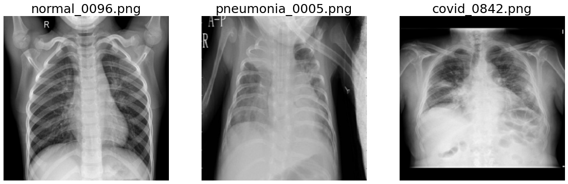
# Display examples
fig, axes = plt.subplots(1, 3, figsize=(20, 12), facecolor="white")
for true_label in Diagnosis:
fnames = [v for v in val_files if true_label.name in os.path.basename(v)]
random.shuffle(fnames)
fname = fnames[0]
im = val_transforms(fname)
ax = axes[true_label.value]
im_show = ax.imshow(im[0], cmap="gray")
ax.set_title(os.path.basename(fname), fontsize=25)
ax.axis("off")
Training
def create_new_net() -> DenseNet121:
    """Create new DenseNet121"""
    return DenseNet121(spatial_dims=2, in_channels=1, out_channels=num_class).to(device)
%matplotlib notebook

max_epochs = 30
val_interval = 1
lr = 1e-5
epoch_loss_values = []
auc = []
acc = []
best_acc = -1

net = create_new_net()
loss = torch.nn.CrossEntropyLoss()
opt = torch.optim.Adam(net.parameters(), lr)
auc_metric = monai.metrics.ROCAUCMetric()

# Plotting stuff
fig, ax = plt.subplots(1, 1, facecolor="white")
ax.set_xlabel("Epoch")
ax.set_ylabel("Metrics")
plt.ion()
fig.show()
fig.canvas.draw()

for epoch in range(max_epochs):
    net.train()
    epoch_loss = 0

    for batch_data in train_loader:
        inputs, labels = batch_data[0].to(device), batch_data[1].to(device)
        opt.zero_grad()
        outputs = net(inputs)
        lossval = loss(outputs, labels)
        lossval.backward()
        opt.step()

        epoch_loss += lossval.item()

    epoch_loss /= len(train_loader)
    epoch_loss_values.append(epoch_loss)

    if (epoch + 1) % val_interval == 0:
        with eval_mode(net):
            y_pred = torch.tensor([], dtype=torch.float32, device=device)
            y = torch.tensor([], dtype=torch.long, device=device)

            for val_data in val_loader:
                val_images, val_labels = (
                    val_data[0].to(device),
                    val_data[1].to(device),
                )

                outputs = net(val_images)
                y_pred = torch.cat([y_pred, outputs], dim=0)
                y = torch.cat([y, val_labels], dim=0)

            y_onehot = [y_trans(i) for i in decollate_batch(y)]
            y_pred_act = [y_pred_trans(i) for i in decollate_batch(y_pred)]
            auc_metric(y_pred_act, y_onehot)
            del y_pred_act, y_onehot
            auc_result = auc_metric.aggregate()
            auc_metric.reset()
            auc.append(auc_result)

            acc_value = torch.eq(y_pred.argmax(dim=1), y)
            acc_metric = acc_value.sum().item() / len(acc_value)
            acc.append(acc_metric)

            if acc_metric > best_acc:
                best_acc = acc_metric
                torch.save(net.state_dict(), os.path.join(root_dir, "best_acc_covid_tutorial.pth"))

    ax.clear()
    train_epochs = np.linspace(1, epoch + 1, epoch + 1)
    ax.plot(train_epochs, epoch_loss_values, label="Avg. loss")
    val_epochs = np.linspace(1, epoch + 1, np.floor((epoch + 1) / val_interval).astype(np.int32))
    ax.plot(val_epochs, acc, label="ACC")
    ax.plot(val_epochs, auc, label="AUC")
    ax.set_xlabel("Epoch")
    ax.set_ylabel("Metrics")
    ax.legend()
    fig.canvas.draw()

/home/local/KHQ/elim.schenck/anaconda3/envs/test/lib/python3.9/site-packages/torch/nn/functional.py:718: UserWarning: Named tensors and all their associated APIs are an experimental feature and subject to change. Please do not use them for anything important until they are released as stable. (Triggered internally at  /pytorch/c10/core/TensorImpl.h:1156.)
  return torch.max_pool2d(input, kernel_size, stride, padding, dilation, ceil_mode)
%matplotlib inline
# Load best model
net.load_state_dict(torch.load(os.path.join(root_dir, "best_acc_covid_tutorial.pth")))
net.to(device)
net.eval()
with eval_mode(net):
y_pred = torch.tensor([], dtype=torch.float32, device=device)
y = torch.tensor([], dtype=torch.long, device=device)
for val_data in val_loader:
val_images, val_labels = (
val_data[0].to(device),
val_data[1].to(device),
)
outputs = net(val_images)
y_pred = torch.cat([y_pred, outputs.argmax(dim=1)], dim=0)
y = torch.cat([y, val_labels], dim=0)
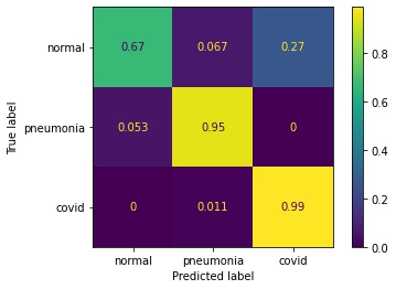
print(classification_report(y.cpu().numpy(), y_pred.cpu().numpy(), target_names=[d.name for d in Diagnosis]))
cm = confusion_matrix(
y.cpu().numpy(),
y_pred.cpu().numpy(),
normalize="true",
)
disp = ConfusionMatrixDisplay(
confusion_matrix=cm,
display_labels=[d.name for d in Diagnosis],
)
disp.plot(ax=plt.subplots(1, 1, facecolor="white")[1])
              precision    recall  f1-score   support

      normal       0.91      0.67      0.77        15
   pneumonia       0.90      0.95      0.92        19
       covid       0.96      0.99      0.97        91

    accuracy                           0.94       125
   macro avg       0.92      0.87      0.89       125
weighted avg       0.94      0.94      0.94       125
<sklearn.metrics._plot.confusion_matrix.ConfusionMatrixDisplay at 0x7fcefd414fd0>
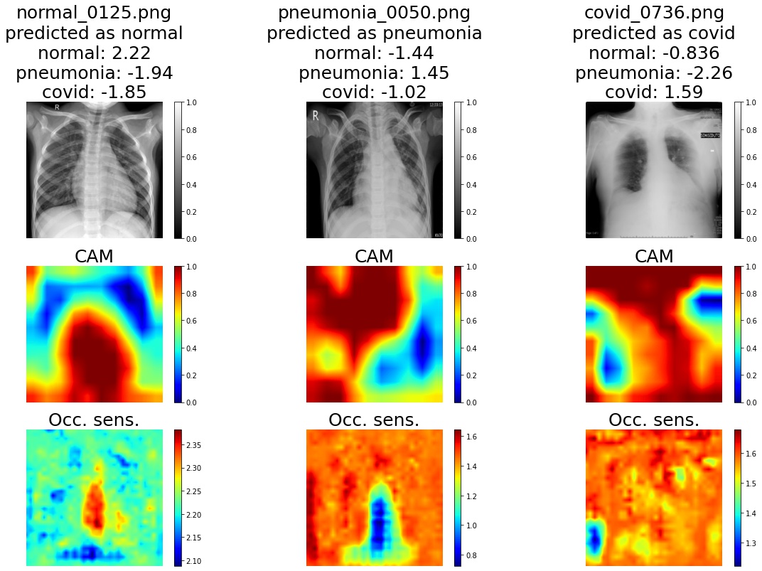
Interpretability Using MONAI
Use GradCAM and occlusion sensitivity for network interpretability.
The occlusion sensitivity returns two images: the sensitivity image and the most probable class.
Sensitivity image – how the probability of an inferred class changes as the corresponding part of the image is occluded.
Big decreases in the probability imply that that region was important in inferring the given class.
The output is the same as the input, with an extra dimension of size N appended. Here, N is the number of inferred classes. To then see the sensitivity image of the class we’re interested in (maybe the true class, maybe the predcited class, maybe anything else), we simply do
im[...,i].
Most probable class – if that part of the image is covered up, does the predicted class change, and if so, to what?
In this example, the network has been sufficiently trained that the predicted class doesn’t change as parts of the image are occluded (so we don’t show the most probable class maps). However, this feature might be useful when the results are less than satisfactory.
# for name, _ in net.named_modules(): print(name)
target_layer = "class_layers.relu"

gradcam = monai.visualize.GradCAM(nn_module=net, target_layers=target_layer)
occ_sens = monai.visualize.OcclusionSensitivity(nn_module=net, mask_size=10, n_batch=batch_size, stride=10)
We can now visualize the computed saliency maps for each image.
# Display examples
subplot_shape = [3, num_class]
fig, axes = plt.subplots(*subplot_shape, figsize=(20, 12), facecolor="white")

for true_label in Diagnosis:
    fnames = [v for v in val_files if true_label.name in os.path.basename(v)]
    random.shuffle(fnames)
    # Find a correctly predicted example
    for fname in fnames:
        img = val_transforms(fname)[None].to(device)
        y_pred = net(img)
        pred_label = Diagnosis(y_pred.argmax(1).item())
        if pred_label == true_label:
            break
    im_title = f"{os.path.basename(fname)}\npredicted as {pred_label.name}"
    for d in Diagnosis:
        im_title += f"\n{d.name}: {y_pred[0, d.value]:.3}"

    res_cam = gradcam(x=img, class_idx=true_label.value)
    occ_map, occ_most_prob = occ_sens(x=img)
    occ_map = occ_map[..., true_label.value]

    # the rest is for visualisations
    for row, (im, title) in enumerate(
        zip(
            [img, res_cam, occ_map],
            [im_title, "CAM", "Occ. sens."],
            strict=False,
        ),
    ):
        cmap = "gray" if row == 0 else "jet"
        col = true_label.value
        ax = axes[row, col]
        if isinstance(im, torch.Tensor):
            im = im.detach().cpu()
            im_show = ax.imshow(im[0][0], cmap=cmap)

        ax.set_title(title, fontsize=25)
        ax.axis("off")
        fig.colorbar(im_show, ax=ax)
Computing occlusion sensitivity: 100%|██████| 1024/1024 [00:13<00:00, 75.62it/s]
Computing occlusion sensitivity: 100%|██████| 1024/1024 [00:12<00:00, 79.02it/s]
Computing occlusion sensitivity: 100%|██████| 1024/1024 [00:12<00:00, 80.44it/s]
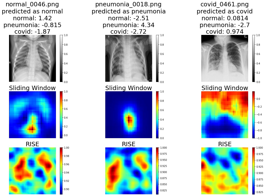
Interpretability Using xaitk-saliency
Using the xaitk-saliency package, we can also compute occlusion-based saliency using either a sliding window approach (similar to the method provided by MONAI) or the RISE saliency algorithm. Here, we will demo the ability to switch out the saliency algorithm.
from smqtk_classifier import ClassifyImage

from xaitk_saliency.impls.gen_image_classifier_blackbox_sal.rise import RISEStack
from xaitk_saliency.impls.gen_image_classifier_blackbox_sal.slidingwindow import SlidingWindowStack

gen_slidingwindow = SlidingWindowStack((50, 50), (20, 20), threads=4)
gen_rise = RISEStack(1000, 8, 0.5, seed=0, threads=4, debiased=False)
We will wrap the COVID model in smqtk-classifier’s ClassifyImage interface for standardized classifier operation with our API.
class COVIDModel(ClassifyImage):
    """Blackbox model based on smqtk-classifier's ClassifyImage."""

    def get_labels(self) -> Sequence[str]:
        """Return a list of Diagnosis labels"""
        return list(Diagnosis.__members__)

    @torch.no_grad()
    def classify_images(self, image_iter: Sequence[np.ndarray]) -> dict[str, Any]:
        """Input may either be an NDaray, or some arbitrary iterable of NDarray images."""

        for img in image_iter:
            img = val_transforms(img)[None].to(device)
            y_pred = net(img)
            # Converting feature extractor output to probabilities.
            class_conf = torch.nn.functional.softmax(y_pred, dim=1).cpu().detach().numpy().squeeze()
            # Only return the confidences for the focus classes
            yield dict(zip(self.get_labels(), class_conf, strict=False))

    def get_config(self) -> dict[str, Any]:
        """Required by a parent class."""
        return {}


blackbox_classifier = COVIDModel()
# Redefine val_transforms here to be able to take in perturbed images if needed
val_transforms = Compose(
    [
        Lambda(lambda s: LoadImage(image_only=True)(s) if isinstance(s, str) else np.array(s)),
        Lambda(lambda im: im if im.ndim == 2 else im[..., 0]),
        AddChannel(),
        Resize(spatial_size=crop_size, mode="area"),
        ScaleIntensity(),
        EnsureType(),
    ],
)
Similarly, we’ll visualize the saliency maps for each image.
# Display examples
subplot_shape = [3, num_class]
fig, axes = plt.subplots(*subplot_shape, figsize=(20, 12), facecolor="white")

for true_label in Diagnosis:
    fnames = [v for v in val_files if true_label.name in os.path.basename(v)]
    random.shuffle(fnames)
    # Find a correctly predicted example
    for fname in fnames:
        img = val_transforms(fname)[None].to(device)
        y_pred = net(img)
        pred_label = Diagnosis(y_pred.argmax(1).item())
        if pred_label == true_label:
            break
    im_title = f"{os.path.basename(fname)}\npredicted as {pred_label.name}"
    for d in Diagnosis:
        im_title += f"\n{d.name}: {y_pred[0, d.value]:.3}"

    # Generate saliency maps
    ref_image = img.cpu().numpy().squeeze()
    sw_sal_map = gen_slidingwindow(ref_image, blackbox_classifier)[true_label.value]
    rise_sal_map = gen_rise(ref_image, blackbox_classifier)[true_label.value]

    # the rest is for visualisations
    for row, (im, title) in enumerate(
        zip(
            [img[0][0], sw_sal_map, rise_sal_map],
            [im_title, "Sliding Window", "RISE"],
            strict=False,
        ),
    ):
        cmap = "gray" if row == 0 else "jet"
        col = true_label.value
        ax = axes[row, col]
        if isinstance(im, torch.Tensor):
            im = im.detach().cpu()
        im_show = ax.imshow(im, cmap=cmap)

        ax.set_title(title, fontsize=25)
        ax.axis("off")
        fig.colorbar(im_show, ax=ax)